« User Manual 3.3 Trigonometric Polynomials and Fourier Series » : différence entre les versions
Aucun résumé des modifications |
|||
| Ligne 262 : | Ligne 262 : | ||
== [[File:lightBulb.png]] Tips & Tricks == | == [[File:lightBulb.png]] Tips & Tricks == | ||
* <code>a</code> and <code>b</code> arrays must have the same lengths! | * <code>a</code> and <code>b</code> arrays must have the same lengths! | ||
[[Category:User_Manual_3.3_Mathematics]] | |||
Version du 27 février 2018 à 14:21
Introduction
Scope
This section presents the Trigonometric Polynomials implemented in PATRIUS as well as Fourier Series.
Javadoc
The trigonometric polynomial (and related) objects are available in the package org.commons.math3.analysis.polynomials in the Commons Math Library (and Commons Math add-ons) and the FFT algorithms inorg.commons.math3.transform
| Library | Javadoc |
|---|---|
| Commons Math add-ons | Package org.commons.math3.geometry.analysis.polynomials |
| Commons Math | Package org.commons.math3.transform |
Links
Useful resources for this theme can be found here :
Useful Documents
Modèle:SpecialInclusion prefix=$theme sub section="UsefulDocs"/
Package Overview

Features Description
Trigonometric Polynomials
The trigonometric polynomials are defined as :
[math]\displaystyle{ \forall t \in \mathbb{R}, P(t) = a_0 + \sum_{k=0}^n \left( a_k \cos(kt) + b_k \sin(kt) \right) }[/math]
And the primitive of such a function is :
[math]\displaystyle{ \forall t \in \mathbb{R}, P(t) = a_0 t + c^{te} + \sum_{k=0}^n \left( {-b_k \over k} \cos(kt) + {a_k \over k} \sin(kt) \right) }[/math]
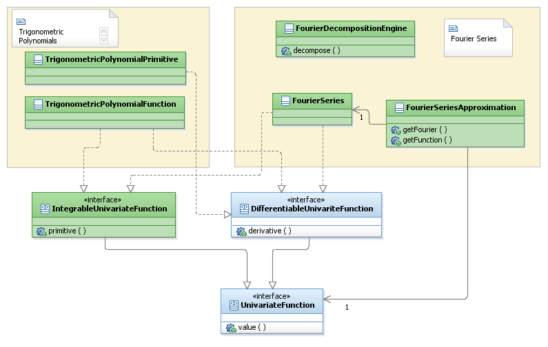
Classes that represent these functions are described in this section.
Fourier Series
Let [math]\displaystyle{ f }[/math] be a periodic, real variable, real function with period [math]\displaystyle{ T }[/math]. The partial sums of the Fourier Series of [math]\displaystyle{ f }[/math] are given by
[math]\displaystyle{ \forall N \in \mathbb{R}^{+*}, \, \left(S_Nf\right)(x) = a_0 + \sum_{n=1}^N\left(a_n\cos\left(n t {2\pi\over T}\right) + b_n\sin\left(n t {2\pi\over T}\right)\right) }[/math]
The Fourier coefficients (n > 0) of [math]\displaystyle{ f }[/math] are given by :
[math]\displaystyle{ a_0 = {1\over T}\int_{-T/2}^{T/2} \! f(t) \, \mathrm{d}t }[/math]
[math]\displaystyle{ a_n = {2\over T}\int_{-T/2}^{T/2} \! f(t) \cos\left(n t {2\pi\over T}\right) \, \mathrm{d}t }[/math]
[math]\displaystyle{ b_n = {2\over T}\int_{-T/2}^{T/2} \! f(t) \sin\left(n t {2\pi\over T}\right) \, \mathrm{d}t }[/math]
Classes that allow decomposing functions into finite Fourier series are described.
Fast Fourier Transforms
A fast Fourier transform (FFT) is an algorithm to compute the discrete Fourier transform (DFT) and its inverse. Fourier analysis converts time (or space) to frequency and vice versa. An FFT rapidly computes such transformations by factorizing the DFT matrix into a product of sparse (mostly zero) factors.
Let [math]\displaystyle{ ( X_0, ..., X_{N-1}) }[/math] be complex numbers. The DFT is defined by the formula
[math]\displaystyle{ X_k = \sum^{N-1}_{n=0} x_n e^{-2i\pi k n/N}, \quad k=\left\{0, ..., N-1\right\}. }[/math]
The class FastFourierTransformer.java owns two methods
transform(final double[] f, final TransformType type)
transform(final Complex[] f, final TransformType type)
where TransformType is an enumeration that defines the type of transform which is to be computed. It can be FORWARD or INVERSE.
Depending on the size, this method will use a radix-2 algorithm if the size is a power-of-two, and the Bluestein algorithm otherwise. Both algorithms are explained above.
The Cooley–Tukey & radix-2 the algorithm
By far the most commonly used FFT algorithm. This is a divide and conquer algorithm that recursively breaks down a DFT of any composite size [math]\displaystyle{ N = N_1N_2 }[/math] into many smaller DFTs of sizes [math]\displaystyle{ N_1 }[/math] and [math]\displaystyle{ N_2 }[/math], along with [math]\displaystyle{ O(N) }[/math] multiplications by complex roots of unity.
The radix-2 algorithme is the most common use of FFT algorithm and is based on the Cooley–Tukey algorithm. It divides the transform into two pieces of size [math]\displaystyle{ N/2 }[/math] at each step, and is therefore limited to power-of-two sizes.
The Bluestein algorithm
It is commonly called the chirp z-transform algorithm. It computes the discrete Fourier transform (DFT) of arbitrary sizes (including prime sizes) by re-expressing the DFT as a convolution. For more information, see [1]
Getting Started
Modèle:SpecialInclusion prefix=$theme sub section="GettingStarted"/
Contents
Interfaces
| Interface | Summary | Javadoc |
|---|---|---|
| DifferentiableUnivariateFunction | Extension of UnivariateFunction representing a differentiable univariate function. | ... |
| IntegrableUnivariateFunction | Extension of UnivariateRealFunction representing an integrable univariate function. | ... |
| DifferentiableIntegrableUnivariateFunction | Extension of UnivariateRealFunction representing a differentiable and integrable univariate function. | ... |
| UnivariateFunction | Interface representing an univariate function. | ... |
| IFastFourierTransformer | Interface representing a FFT. | ... |
Classes
| Class | Summary | Javadoc |
|---|---|---|
| FourierDecompositionEngine | Decompose a UnivariateFunction as a Fourier Series using TrigonometricPolynomialFunction representation. | ... |
| FourierSeries | This class represents a finite Fourier Series. | ... |
| FourierSeriesApproximation | Holder for a UnivariateFunction and its FourierSeries approximation. | ... |
| TrigonometricPolynomialFunction | This class is the Trigonometric Polynomial Function class. | ... |
| TrigonometricPolynomialPrimitive | This class represents a Trigonometric Polynomial Primitive. | ... |
| AbstractFastFourierTransformer | Abstract class representing a FFT. | ... |
| FastFourierTransformer | Computes the FFT for real and complex arrays. | ... |
Usage of a trigonometric polynomial
- To create the polynomial [math]\displaystyle{ P(x) =-2 + \cos(x) + 2\sin(3x) }[/math], use the following code snippet :
double a0 =-2;
double[] a = new double[] {1, 0, 0};
double[] b = new double[] {0, 0, 2};
TrigonometricPolynomialFunction myPol2 = new TrigonometricPolynomialFunction(a0, a, b);
- To get the value of the second derivative at [math]\displaystyle{ x = 5 }[/math], use the following snippet :
double result = myPol2.value(2,5);
// equivalent to
double result = myPol2.polynomialDerivative(2).value(5);
- To get the primitive :
// With an integration constant c = 1 :
TrigonometricPolynomialPrimitive result = myPol2.polynomialPrimitive(1.);
- To multiply two trigonometric polynomials [math]\displaystyle{ p1 }[/math] and [math]\displaystyle{ p2 }[/math] :
TrigonometricPolynomialFunction result = p1.multiply(p2);
Decomposing a UnivariateFunction into a Fourier Series
Given a user function with period T :
UnivariateFunction f = new UnivariateFunction () {
    public double value(double x) {
         // ...
         return result;
    }
};
The user must build an instance of the FourierDecompositionEngine (using an integrator) :
FourierDecompositionEngine engine = new FourierDecompositionEngine( integrator );
And pass the function, period and approximation order to it.NOTE : It is left up to the user to make sure that the specified period is coherent with the function as no internal check is conducted.
engine.setOrder(10);
engine.setFunction(f, T);
Then, the user can call the decompose( ) method :
FourierSeriesApproximation approximation = engine.decompose();
FourierSeries fourier = approximation.getFourier();
Example
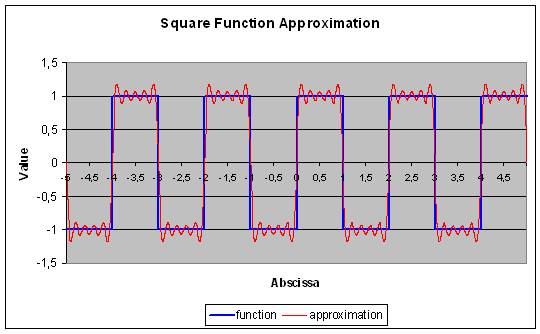
The following code snippet shows how to decompose a square function of period 2 to the 10th order :
// function definition
UnivariateFunction function = new UnivariateFunction() {
   public double value(final double x) {
   final double local = x- FastMath.floor(x / 2) * 2;
      if (local >= 1) {
         return-1;
      } else {
         return 1;
      }
   }
};

// Engine parameters
UnivariateIntegrator integrator = new LegendreGaussIntegrator(5, 1e-14, 1e-14);
FourierDecompositionEngine engine = new FourierDecompositionEngine(integrator);
engine.setMaxEvals(Integer.MAX_VALUE);

// decompose
double period = 2;
engine.setOrder(10);
engine.setFunction(function, period);
FourierSeriesApproximation result = engine.decompose();
FourierSeries fourier = result.getFourier();
The function and its approximation are shown hereunder. The parasite undulations are known as the Gibbs Phenomenon :

Tutorials
Tutorial 1
Modèle:SpecialInclusion prefix=$theme sub section="Tuto1"/
Tutorial 2
Modèle:SpecialInclusion prefix=$theme sub section="Tuto2"/
 Tips & Tricks
aandbarrays must have the same lengths!